A Thesis on Implied Correlation and the College List
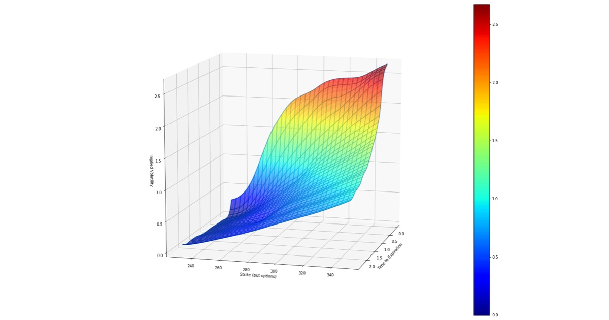
A client's father came in last spring with fourteen schools on a page. Eight of them admit under ten percent. He had done the arithmetic on the drive over and he was pleased with it: eight shots at roughly one in ten, something has to land. Surely his son was going to be fine!
His arithmetic passed the first check. But his model was wrong, and the error has a name in a field he did not work in.
I wrote this piece as a mathematical exploration of admissions strategies in the lens of betting and portfolio theory, something you will never see on any other consulting firm's website. Nearly everything written about admissions is qualitative, and nearly all of it concerns the parts of the process you control least: what a committee will think, whether a reader connects with your voice, how your file reads at four in the afternoon in February. Meanwhile the one decision a family owns outright, the list itself, gets handled as a matter of taste. Pick a few reaches. Add some safeties. Feel it out. The world does not need more of that recycled, scripted crap.
It is not a matter of taste. Choosing what to put on that page is portfolio construction under correlated risk, and portfolio construction under correlated risk is a solved problem. Solved somewhere else, by people who spend their careers pricing the difference between fourteen bets and one bet made fourteen times, and who learned what it costs to confuse the two. The tools have existed for decades. Nobody has bothered to point them at a kitchen table in August.
So this is admissions under a purely statistical lens, and the claim is narrow. The most expensive mistake in this process is not a weak essay or a missed deadline. It is a modeling error, made in August, invisible until March, and an industry built on qualitative advice has no vocabulary to name it.
Count is not in the formula
Take an index of assets with weights and volatilities . Writing out the variance of the weighted sum:
where is the average pairwise correlation. Collect the two pieces. Call the idiosyncratic sum and the pairwise sum :
and the whole thing collapses to:
Read what is missing. There is no term for . Five hundred names at carry the risk of one name. The basket is not doing the work; the cancellation is doing the work, and cancellation is purchased entirely with correlation.
It is worth seeing how hard that bites. Take the equal-weighted case, where every , every , and the pairwise correlation is a constant :
Let run to infinity, infinite names and perfect breadth, and index volatility still does not go to zero. It goes to . There is a floor, and diversification cannot get under it, and the floor is set by correlation alone. You can add names forever and never reach certainty. You reach and stop.
This is why implied correlation is a traded quantity rather than a curiosity. Compare the implied vol of an index against the weighted implied vols of its constituents and you can back out the correlation the market is charging for. Dispersion trades exist to take a view on exactly that number: short index variance, long the components, a bet that things cancel more than the market has priced.
Now put the fourteen schools back on the table.
The ninth school
Before the list, one more property of that formula, because it is the one that changes what you should actually do.
Diversification does not bleed away linearly as rises. Since :
The derivative decays on the order of . Moving correlation from negative or zero to mildly positive produces a large jump in index vol and destroys most of the diversification benefit at once. Moving from 0.8 to 0.9 barely registers. At 0.8 the components were already in near lockstep, and there was little left to take.
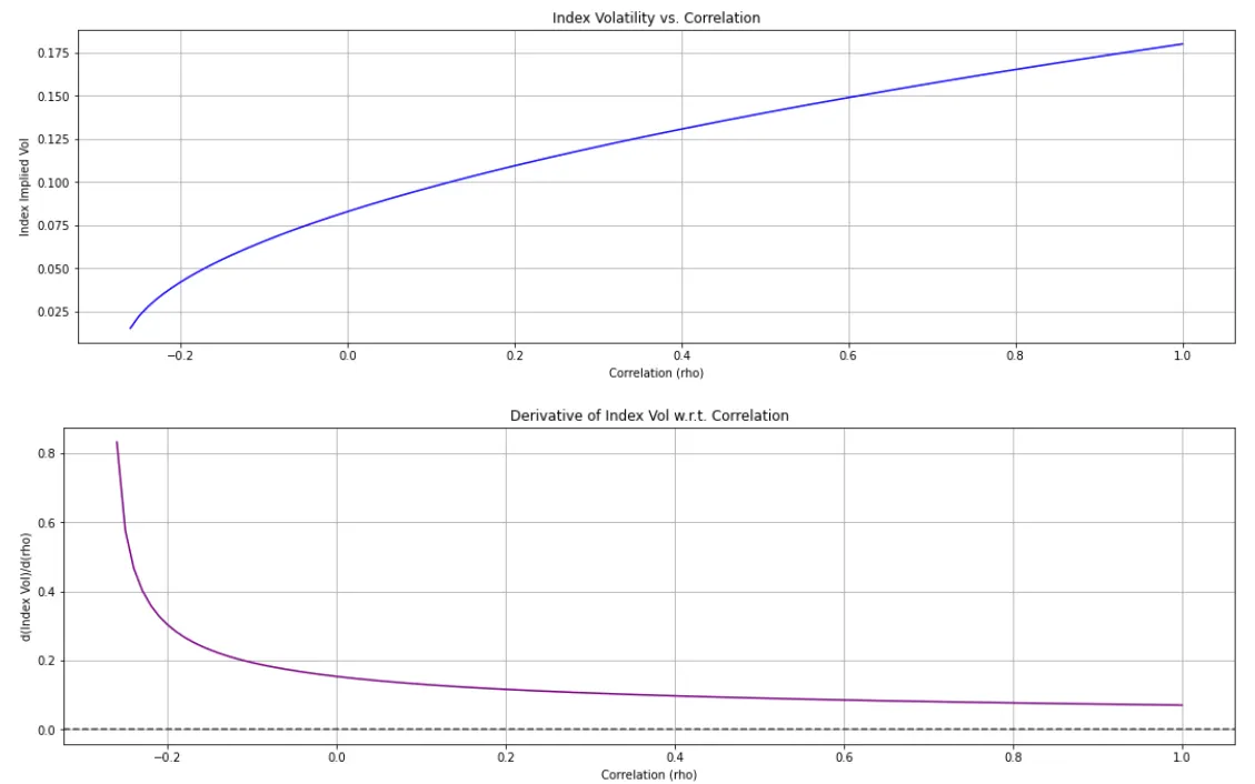
The bottom panel is the whole argument in one line. The sensitivity craters early and is nearly flat past . Once you are out on that flat stretch, more correlation costs almost nothing, and, read the other direction, more names buy almost nothing.
The list is an index
Each application is a component. But the underlying is not fourteen assets. It is one student. That single fact is the whole essay.
The father's calculation assumed independence. Under independence, eight schools at five percent each is genuinely encouraging:
A third of the time, something lands. That is the number in every parent's head, whether or not they could write it down, and it is why add another reach feels like strategy rather than superstition.
But the dice are welded together. Every school reads the same transcript, the same scores, the same activities section, and, small variations aside, the same essays. The readers were trained in overlapping traditions and are looking for overlapping things. If one committee concludes strong, diligent, indistinguishable from four hundred other computer science applicants, the next committee is not running an independent trial. It is re-running the same trial on the same input.
The schools are not even strictly at arm's length. Amherst's dean of admission told U.S. News that Amherst and roughly thirty other colleges shared lists of the students they admitted through early decision, and of those who then did not enroll. The Justice Department opened an antitrust investigation into that kind of coordination in 2018, sued the National Association for College Admission Counseling in 2019, and forced three recruiting rules out of its ethics code. It is not the first time: the Ivies and MIT ran an "Overlap Group" that coordinated aid awards for jointly admitted students until the DOJ sued in 1991. Yield is a shared institutional interest, and institutions with shared interests have a long documented history of comparing notes. Whatever else this process is, it is not a set of independent trials.
I can do better than assert that.
A one-factor model of your file
Give each school a latent evaluation , meaning everything that school thinks about you compressed into a number. The school admits when that number clears its bar . Decompose the evaluation into what every reader sees and what only that reader sees:
is you: the common factor. Your transcript, your essays, your recommenders, the shape of your profile. It is in every envelope, and it does not get resampled. is everything specific to one school: the reader's afternoon, an institutional need, a program that happens to want your thing. And is the share of the decision driven by the part of you that every school sees identically.
If each school admits with unconditional probability , then the bar sits at . Condition on your draw of , which is to say condition on the file you actually have, and the schools become independent:
so the probability of at least one acceptance across schools is:
This is the one-factor Gaussian copula, the standard workhorse for correlated defaults in a credit portfolio. The mapping is not decorative. A pool of loans fails together when the economy turns; a list of applications fails together when the file is the problem. Same structure, same integral.
Evaluate it for eight schools at five percent:
| Correlation | P(at least one admit) |
|---|---|
| 0.0 | 33.7% |
| 0.2 | 29.1% |
| 0.4 | 24.3% |
| 0.6 | 19.4% |
| 0.8 | 14.1% |
| 0.9 | 10.9% |
| 1.0 | 5.0% |
At the model returns 33.7%, exactly reproducing the closed form above, which is the check that it is the same object viewed honestly.
Nobody knows the true for a college list. But consider what is actually shared across those eight envelopes (one transcript, one set of scores, one personal statement, one slate of recommenders, readers trained alike) and ask whether that looks like 0.2 or like 0.7. The father priced his list at 0. The honest range is not close.
Why more schools does not rescue it
Hold fixed and let grow. This is the move every anxious family makes in October.
| Schools | ||
|---|---|---|
| 4 | 18.5% | 13.3% |
| 8 | 33.7% | 19.4% |
| 12 | 46.0% | 23.5% |
| 20 | 64.2% | 29.0% |
Under independence, going from eight schools to twenty nearly doubles your odds, 33.7% to 64.2%. Under a plausible correlation, the same twelve extra applications move you from 19.4% to 29.0%. You did two and a half times the work for less than a third of the promised gain.
And it is worse than the table suggests, because those twelve applications are not free. They cost supplements you do not have time for, slots in a counselor's queue you share with three hundred people, and the attention that the eight schools you actually cared about needed. The father was not one school short of a solution. He held one position, levered eight ways, and called it a portfolio. And say goodbye to $80 to each additional school you apply to.
Skew, or: correlation is not a constant
Here is the part that should genuinely worry you, and it is the reason index options are priced the way they are.
is not a fixed parameter sitting politely in the model. It is state-dependent, and the dependence is vicious: correlation rises in the bad state. In a crash, everything sells off together, and the careful cancellation you paid for evaporates at exactly the moment you were relying on it. Diversification is a fair-weather asset.
That asymmetry is why index skew is steeper than the skew of the constituents. Index puts trade rich relative to a basket of single-name puts, and the premium is not irrational. It is the market pricing the fact that in the downside scenario, . Reconciling index put prices with aggregated constituent put prices requires a higher implied correlation on the downside. Index skew is, in part, correlation risk wearing a different hat.
Point that at the list.
The upside states are idiosyncratic. When you get in somewhere, it is often for a reason peculiar to that school: a program that wanted you, a reader who connected, a year when they needed your thing. Good outcomes are outcomes. They decorrelate.
The downside state does not behave that way at all. Suppose your file has a systematic weakness: an essay that reads as a résumé with feelings, a profile that is strong and utterly interchangeable, a gap between what you claim to care about and what you did. That weakness is not sampled independently by fourteen committees. It is in . Every reader sees the same thing, they reach the same conclusion, and they reach it in the same three weeks of March.
So your list runs low-ish correlation when things go well and close to when they do not. The list is short a correlation spike in the only state it was built to protect against. The families destroyed in March are not the ones who made a bad bet. They are the ones who made one bet fourteen times and only discovered it was one bet when it went against them.
The 5% was never your number
A second error compounds the first, and it is a confusion of measures.
A published admit rate is a pool statistic, not a personal one. Five percent describes a population containing recruited athletes cleared before they applied, development cases, and thousands of applicants with no realistic chance who applied anyway. You are none of them. Your probability conditional on your actual file, which in the language above means conditional on your , is a different number, and it may sit well above or well below the printed one.
The distinction is the one separating a risk-neutral density from a physical one. The implied distribution you read off a market is not the real-world distribution of outcomes; it is a pricing measure. Reading it as a forecast is a beginner's error with expensive consequences.
The father made both errors in sequence: he took a pool-level statistic, read it as his son's probability, and then treated eight draws from it as independent. Two measure errors, stacked, both invisible, both flattering.
Lowering rho
If the binding constraint is , the answer is not volume. It is finding decisions that turn on rather than on .
Two applications are correlated when they rank you on the same axis. If every school sorts on rigor, scores, and the prestige of your activities, you have one bet. To lower , you need evaluations that depend on something the others are not looking at.
- Schools that weight factors differently. Checkable, not intuited. Every college publishes a Common Data Set, and section C7 states how heavily it weighs essays, character, rigor, and the rest. The ratings vary more than families expect. Some schools rate character very important; others do not consider it at all. Those two are not running the same evaluation, which is precisely what makes them different bets.
- Different points of entry. A direct-admit engineering program and a liberal arts college are two evaluations, not one repeated.
- Different rounds. Early and regular are distinct pools with distinct competition, not one pool sampled twice.
- Actual fit. The least quantitative item and the most decorrelating. A school that wants your specific combination is making a judgment the other seven are not equipped to make.
None of these is apply to more schools. Every one is apply to schools asking a different question. A dispersion trader is long the components and short the index because the entire edge lives in what makes each name unlike the basket. The student version of that trade is a list where your is the thing being priced, rather than your rank on an axis with four hundred people stacked on it.
The objections
This argument attracts a handful of serious rebuttals, and two of them are good enough that I think they are right. They all deserve the strongest version of themselves rather than a strawman, so here they are, with the best answer I have.
"You invented . The entire piece rests on a parameter nobody can observe."
Correct, and it is the right place to attack. There is no data feed for the correlation between admissions committees. I cannot estimate the way a desk estimates implied correlation from listed option prices, because the applications are not traded and the decisions are not published.
But the conclusion does not require knowing . It requires knowing it is not zero, and that is not in doubt, because I can enumerate what is literally shared across the envelopes. One transcript. One set of scores. One personal statement. One slate of recommenders. Look again at the table: every value of above zero moves you the same direction, and the collapse is steep and early. The claim is not your odds are exactly 19.4%. The claim is your odds are not 33.7%, and the gap is large, and it does not depend on pinning down the parameter. A model that gives you the sign and the rough size of an error is doing its job even when it cannot give you the third decimal.
"Students get split decisions constantly. Admitted at one, rejected at a peer school. That is evidence the bets are independent."
It is evidence that , which nobody disputes. It is not evidence that .
Look at what the model actually predicts. At , high correlation by any standard, an applicant conditioned on a good draw of still gets a mix of outcomes, because has not vanished. Split decisions are precisely what moderate-to-high correlation looks like from the inside. The anecdote everyone reaches for, my friend got into Harvard and rejected from a school ranked twenty spots lower, is fully consistent with and tells you almost nothing. In fact, run it backwards: the observed frequency of split outcomes among similar applicants is an estimator of . Splits are not the refutation. They are the measurement.
"Correlation cuts both ways. If is high and the file is strong, the student sweeps. You are only telling the scary half."
This is the best objection on the list, and it is right. High correlation does raise the probability of a sweep. Here is the whole distribution rather than the half that suits us:
| P(0 admits) | P(all 8) | E[number of admits] | |
|---|---|---|---|
| 0.0 | 66.3% | 0.0000% | 0.400 |
| 0.3 | 73.3% | 0.0031% | 0.400 |
| 0.6 | 80.6% | 0.1451% | 0.400 |
| 0.9 | 89.1% | 1.5165% | 0.400 |
| 1.0 | 95.0% | 4.9978% | 0.400 |
Read the last column first. The expected number of admits is 0.400 at every level of correlation. It does not move. By linearity of expectation it cannot: regardless of how the indicators are coupled. Correlation has no effect whatsoever on how many acceptances you should expect.
What it does is hollow out the middle. As rises, both tails inflate: the probability of a clean sweep goes from effectively zero to five percent, and the probability of nothing at all goes from 66% to 95%. Same mean, redistributed into a bimodal shape.
So the objection is conceded and it does not rescue the plan. Correlation is not costing you expected admissions. It is costing you the insurance, and insurance was the entire reason the list had fourteen names on it. The father was not buying expected value; was fixed the moment he chose eight schools at five percent. He was buying the reduction in variance that turns 0.4 expected admits into at least one, probably. That is the product correlation quietly takes off the shelf while leaving the price tag on.
Yes, a strong file sweeps. But you do not know your draw of when you build the list in August, and every family silently assumes they are in the right tail. The ones who sweep were going to be fine under any list construction. The list exists for the other branch.
"Then just add a pile of safeties. Schools the kid cannot possibly be rejected from. Problem solved."
This one is correct, and it is worth showing why the model agrees rather than pretending it does not.
Go back to the extreme case. At , the entire list behaves as a single school, so the probability of at least one acceptance is exactly . Now notice what that means at different values of :
| Each school's | ||
|---|---|---|
| 5% | 33.7% | 5.0% |
| 30% | 94.2% | 30.0% |
| 95% | 100.0% | 95.0% |
At five percent, correlation is a catastrophe. At ninety-five percent, correlation costs you essentially nothing. You still get ninety-five percent in the worst case the model can construct.
The reason is worth stating plainly, because it is the cleanest statement of the whole idea. Correlation destroys diversification, and diversification is the machinery that carries you from a small to a large . If a single bet is already close to certain, you were never running that machinery. There is nothing there to break. A safety does not defeat the correlation problem. It never had the problem.
So the honest prescription is not add reaches and it is not add a hundred safeties. It is that one or two real safeties do the entire job, and the twelfth reach does close to nothing, and most families have that backwards.
Three things keep this from being a free lunch.
First, the ninety-five percent is unconditional. It is the average across every version of you, and you only get one. Condition on a weak draw of and it sags:
| Your file | A "95% safety" actually admits |
|---|---|
| average | 99.5% |
| 1 SD weak | 91.6% |
| 2 SD weak | 56.0% |
| 3 SD weak | 14.2% |
The same mechanism as before: it fails in the state where you needed it. In fairness to the objection, constant across schools is the model's weakest assumption right here. A genuine safety turns mostly on numbers you can already see, so the real residual uncertainty is smaller than that table suggests. Do not take the 14.2% literally. Take the direction.
Second, a safety's probability is not even increasing in how strong you are. Schools protect their yield, and an applicant who reads as certain to enroll elsewhere can be waitlisted for that reason alone. Your safety is safest when it believes you.
Third, and most importantly, it answers a question nobody asked. The father was not buying a college. Anyone can have a college. He was buying a shot at those eight, and a safety does nothing for that. It buys a floor. Floors are worth having, and a floor is not the thing he drove over to talk about.
"This is 'build a balanced list' dressed up in Greek letters."
It is close to the opposite, and the difference is the practical payload.
Conventional advice operates on . Add safeties, add targets, lower the average admit rate you are facing. That advice is not wrong, but it is blind to , and is a separate dial. Two schools with identical five percent admit rates can be radically different bets depending on whether they evaluate the same axis. Standard tiering has no way to express that, because it sorts schools by difficulty and never by what question they ask.
Which is why the recommendation lands somewhere tiering never does. It is not add more schools and it is not add easier schools. It is add schools whose decision turns on a different part of you. And, uncomfortably for us, it implies doing fewer applications more deliberately, which is less work for a family to buy and less revenue for anyone selling application help by the unit.
One caveat I will not paper over: the one-factor Gaussian copula is a modeling convenience, not a theory of how committees think. Nobody in an admissions office computes a latent variable. But nothing in the conclusion depends on Gaussianity or on thresholds. Any model in which a shared component drives a meaningful share of the decision produces the same shape, because the shape comes from the sharing, not from the distribution. The math is a way to see the structure. The structure was there before the math showed up.
"Admissions is holistic. Human. You cannot reduce a person to a number, and it is a little grotesque to try."
I have saved this one for last because it is the objection people feel most strongly, and because it has the answer with the sharpest edge.
The institution on the other side of the table reduced you to a number a long time ago.
Enrollment management is a mature industry with vendors, conferences, and a price list. Firms like Ruffalo Noel Levitz and Maguire Associates built their business on analyzing an applicant's price sensitivity and ability to pay in order to construct targeted offers. Universities buy predictive yield models that estimate the probability a given admit enrolls, then run what-if simulations on aid packages before the awards go out, tuning net tuition revenue against class size. Financial aid optimization is a product you can purchase. There are case studies with named universities and reported yield gains.
I mean, the Duke University endowment publicly discloses what their internal hedge fund invests in every few years, along with their performance. You think their $12 billion dollar endowment (which included tons of speculative assets like Ethereum) cares about your common app?
Think about what that machinery has to solve. The office cannot simply admit the best applicants. It has to land a class of a specific size, because there are that many beds and that many seats in the introductory sequence. It needs the majors to distribute so the department that can teach four hundred students does not receive nine hundred. It needs the discount rate to come in on budget. It needs enough of the class to actually show up in September. Those are constraints, and hitting several at once across tens of thousands of applicants with uncertain yield is an optimization problem. It is solved the way optimization problems are solved, by people hired to solve them.
Now hold that next to the argument that this cannot be modeled.
It is already being modeled. It is being modeled by professionals, continuously, with better data than you will ever have, and the output of those models is the environment you are applying into. The reader who opens your file is real, and thoughtful, and probably cares. They are also an input to a process whose objective function they did not write and, in most cases, have never seen. When a strong applicant is waitlisted for looking too likely to go elsewhere, no human decided the student was unworthy. A yield constraint decided it.
So the asymmetry is not between people who use math and people who respect the humanity of the process. Both sides are running on numbers. The asymmetry is that one side has quantitative staff and the other side has a father doing arithmetic in the car.
I am not arguing that a person is a number. I am contending that a list is a portfolio, which it plainly is, and that refusing to think about it quantitatively does not make the process more human. It just means you are the only one at the table who brought nothing.
What this does not fix
Lowering does not deliver 33.7%. Nothing does. There is a floor, just as was a floor, and the honest ceiling on a list of highly selective schools is lower than any family wants to hear.
What it fixes is the illusion, and the illusion is the expensive part. The father drove in with a plan whose expected outcome he had overstated by roughly a factor of six, and he could not see the failure mode, because the arithmetic on the drive over was correct. That is the dangerous species of wrong. Not sloppy. Rigorous-looking.
Count is not in the formula. Correlation is in the formula. It is true of the S&P 500 and it is true of the fourteen schools on your kitchen table, and it is highest at exactly the moment you need it lowest.
If you want a second read on whether your list is fourteen bets or one bet in fourteen costumes, that is a good deal of what we do this time of year. Apply to work with us via a free consultation.